library(dplyr)
library(ggplot2)
library(tidyverse)
library(maptools)
library(leaflet)
library(RColorBrewer)
library(rworldmap)
library(sp)

GDP and Forest Data Management

Gross Domestic Product (GDP) is displayed as an economic development indicator as Percent of Total Land Forested was selected to evaluate trends in forest biomass in the region. Both of these variables are found in data that is drawn from the World Bank Group. The package dplyr is used to taylor the data to regional characteristics. The tables are designed to display simple characteristic change over time.

download.file("http://api.worldbank.org/v2/en/indicator/NY.GDP.MKTP.CD?downloadformat=csv",destfile = "data/GDP.zip")
unzip("data/GDP.zip",exdir = "data")
GDP<-read.csv("data/API_NY.GDP.MKTP.CD_DS2_en_csv_v2.csv",skip=4)


GDP_filter<-dplyr::filter(GDP,GDP$Country.Name=="Thailand"|GDP$Country.Name=="Cambodia"|GDP$Country.Name=="Vietnam"|GDP$Country.Name=="Myanmar"|GDP$Country.Name=="Lao PDR")
GDP_subset<-subset(GDP_filter,select=-c(5:49,61:62)) 

GDP_G<-gather(GDP_subset,"Year","GDP",5:15)%>%
  mutate(Year=(sub("X","",Year)))


download.file("http://api.worldbank.org/v2/en/indicator/AG.LND.FRST.ZS?downloadformat=csv",destfile = "data/forest.zip")
unzip("data/forest.zip",exdir = "data")
Forest_data<-read.csv("data/API_AG.LND.FRST.ZS_DS2_en_csv_v2.csv",skip=4)


Forest_filter<- dplyr::filter(Forest_data,Forest_data$Country.Name=="Thailand" |Forest_data$Country.Name=="Cambodia"|Forest_data$Country.Name=="Vietnam"|Forest_data$Country.Name=="Myanmar"|Forest_data$Country.Name=="Lao PDR")
For_subset<-subset(Forest_filter,select=-c(5:49,61:62)) 

Forest_G<-gather(For_subset,"Year","Forest",5:15)%>%
  mutate(Year=(sub("X","",Year)))

plotcolors=c("#1b9e77", "#d95f02", "#7570b3", "#e7298a", "#66a61e")

These tables created above are joined by the “Country.Name” variable to create a comparison table of GDP and Percent of Forested Land.

GDP and Forest Change join

GDPF_join=left_join(GDP_G,Forest_G,by=c("Country.Name","Year"))

GDPF_plot=ggplot(GDPF_join,aes(x=GDP,y=Forest,group=Country.Name))

World Comparison Map

Using leaflet, I generated an interactive map displaying total percentage of forest loss over a ten year period (2005-2015). To do this I had to collect data of forest loss from Global Forest Watch. A 50% Tree Cover Canopy was selected from the data. Tree Cover Canopy (TCC), corrosponds to density of tree cover before loss occured estimated by remotely sensed pixels (Hansen et.al). Global Forest Watch suggests 50% TCC data is most representative for each country.

TCstats=readxl::read_xlsx("data/TCstats.xlsx","Loss (2001-2016) by Country",skip=1)

TCsub=subset(TCstats,select=(c(1,6:16,91:101,108:118)))                               

TCFilter=filter(TCsub,TCsub$Country=="Thailand"|TCsub$Country=="Cambodia"|TCsub$Country=="Vietnam"|TCsub$Country=="Myanmar"|TCsub$Country=="Laos")


W_agg=select(TCsub,1,13:23)
W_agg$totalsum=rowSums(W_agg[,-1])

I then had to retrieve total (not percent) land area forested, which is measured in km^2, from the World Bank. Due to different data origins, many country names from the World Bank Data had to be manually renamed for a successful join of the datasets. After the join, the ten year total of forest loss was divided by the ten year total of forested land area of each country. This value was multiplied by 100 to make the value a percentage. The new dataset was spatial joined by using the package rworldmap.

download.file("http://api.worldbank.org/v2/en/indicator/AG.LND.FRST.K2?downloadformat=csv",destfile="data/Forestareatotal.zip")
unzip("data/Forestareatotal.zip",exdir = "data")
FA_total=read.csv("data/Forestareatotal/API_AG.LND.FRST.K2_DS2_en_csv_v2.csv",skip = 4)

FAT_sel=select(FA_total,1,50:60)
FAT_sel$Country.Name=as.character(FAT_sel$Country.Name)
FAT_sel[128,1]="Laos"
FAT_sel[201,1]="Russia"
FAT_sel[111,1]="Iran"
FAT_sel[66,1]="Egypt"
FAT_sel[42,1]="Democratic Republic of the Congo"
FAT_sel[220,1]="Slovakia"
FAT_sel[253,1]="Venezuela"
FAT_sel[43,1]="Republic of Congo"
FAT_sel[261,1]="Yemen"
FAT_sel[121,1]="Kyrgyzstan"
FAT_sel[226,1]="Syria"



# Multiplied by 100 to convert area in kms^2 to hectares
FAT_sel$areasum=rowSums(FAT_sel[,-1])
FAT_sel$Hectarea=FAT_sel$areasum*100


colnames(FAT_sel)[colnames(FAT_sel)=="Country.Name"] <- "Country"
Wag_Fat_join=left_join(W_agg,FAT_sel,by="Country")
JN=mutate(Wag_Fat_join,tloss=(totalsum/Hectarea)*100)
JN_join=joinCountryData2Map(JN,joinCode = "NAME",nameJoinColumn = "Country")

## 227 codes from your data successfully matched countries in the map
## 29 codes from your data failed to match with a country code in the map
## 16 codes from the map weren't represented in your data

After the spatial join I set bin values that would best display the data. The bin values have small divisions as most of the values were assigned at a fraction of a percent. Criteria for color scale and labeling are also set in this step.

bins <- c(0,0.5, 1,5,10,15,20,Inf)
pal <- colorBin("Reds", domain = na.omit(JN_join$tloss), bins = bins)

web_map=leaflet(JN_join)%>%
  addProviderTiles(providers$CartoDB.Positron)


TCWebmap=web_map%>%
  addPolygons(fillColor = ~pal(tloss),
              fillOpacity = 0.7, 
              weight=1,
              color="grey",
              highlight=highlightOptions(weight=3, 
              color="#666",bringToFront=TRUE),
              label=paste(JN_join$Country,round(JN_join$tloss,2),"% forested area lost"))

Displaying Change Over Time

Next, I want to display a yearly change in forest loss based upon total Hectares lost by country by year. First I had to create new tables to have each country have a uniform Year column name for a join. I also had to mutate the Year column to give each country a “Year” value.

Yearlytot=gather(FAT_sel,"Year","Area",2:12)%>%
  mutate(Year=sub("X","",Year))
Yearlyloss=gather(W_agg,"Year","Loss",2:12)%>%
  mutate(Year=sub("__5","",Year))


Year_join=left_join(Yearlytot,Yearlyloss,by=c("Year","Country"))
Year_join$Harea=Year_join$Area*100
YJN=mutate(Year_join,losspercent=(Loss/Harea)*100)

I then had to go through the newly joined table and use dplyr to filter out each country in the study area for every year from 2005 to 2015. After the filter of the dataset, each year had to be individually spatial joined.

SEA_Year_05=filter(YJN,YJN$Country=="Thailand"|YJN$Country=="Cambodia"|YJN$Country=="Vietnam"|YJN$Country=="Myanmar"|YJN$Country=="Laos",YJN$Year=="2005")

SEA_Year_06=filter(YJN,YJN$Country=="Thailand"|YJN$Country=="Cambodia"|YJN$Country=="Vietnam"|YJN$Country=="Myanmar"|YJN$Country=="Laos",YJN$Year=="2006")

SEA_Year_07=filter(YJN,YJN$Country=="Thailand"|YJN$Country=="Cambodia"|YJN$Country=="Vietnam"|YJN$Country=="Myanmar"|YJN$Country=="Laos",YJN$Year=="2007")

SEA_Year_08=filter(YJN,YJN$Country=="Thailand"|YJN$Country=="Cambodia"|YJN$Country=="Vietnam"|YJN$Country=="Myanmar"|YJN$Country=="Laos",YJN$Year=="2008")

SEA_Year_09=filter(YJN,YJN$Country=="Thailand"|YJN$Country=="Cambodia"|YJN$Country=="Vietnam"|YJN$Country=="Myanmar"|YJN$Country=="Laos",YJN$Year=="2009")

SEA_Year_10=filter(YJN,YJN$Country=="Thailand"|YJN$Country=="Cambodia"|YJN$Country=="Vietnam"|YJN$Country=="Myanmar"|YJN$Country=="Laos",YJN$Year=="2010")

SEA_Year_11=filter(YJN,YJN$Country=="Thailand"|YJN$Country=="Cambodia"|YJN$Country=="Vietnam"|YJN$Country=="Myanmar"|YJN$Country=="Laos",YJN$Year=="2011")

SEA_Year_12=filter(YJN,YJN$Country=="Thailand"|YJN$Country=="Cambodia"|YJN$Country=="Vietnam"|YJN$Country=="Myanmar"|YJN$Country=="Laos",YJN$Year=="2012")

SEA_Year_13=filter(YJN,YJN$Country=="Thailand"|YJN$Country=="Cambodia"|YJN$Country=="Vietnam"|YJN$Country=="Myanmar"|YJN$Country=="Laos",YJN$Year=="2013")

SEA_Year_14=filter(YJN,YJN$Country=="Thailand"|YJN$Country=="Cambodia"|YJN$Country=="Vietnam"|YJN$Country=="Myanmar"|YJN$Country=="Laos",YJN$Year=="2014")

SEA_Year_15=filter(YJN,YJN$Country=="Thailand"|YJN$Country=="Cambodia"|YJN$Country=="Vietnam"|YJN$Country=="Myanmar"|YJN$Country=="Laos",YJN$Year=="2015")


join_05=joinCountryData2Map(SEA_Year_05,joinCode = "NAME",nameJoinColumn = "Country")

## 5 codes from your data successfully matched countries in the map
## 0 codes from your data failed to match with a country code in the map
## 238 codes from the map weren't represented in your data

join_06=joinCountryData2Map(SEA_Year_06,joinCode = "NAME",nameJoinColumn = "Country")

## 5 codes from your data successfully matched countries in the map
## 0 codes from your data failed to match with a country code in the map
## 238 codes from the map weren't represented in your data

join_07=joinCountryData2Map(SEA_Year_07,joinCode = "NAME",nameJoinColumn = "Country")

## 5 codes from your data successfully matched countries in the map
## 0 codes from your data failed to match with a country code in the map
## 238 codes from the map weren't represented in your data

join_08=joinCountryData2Map(SEA_Year_08,joinCode = "NAME",nameJoinColumn = "Country")

## 5 codes from your data successfully matched countries in the map
## 0 codes from your data failed to match with a country code in the map
## 238 codes from the map weren't represented in your data

join_09=joinCountryData2Map(SEA_Year_09,joinCode = "NAME",nameJoinColumn = "Country")

## 5 codes from your data successfully matched countries in the map
## 0 codes from your data failed to match with a country code in the map
## 238 codes from the map weren't represented in your data

join_10=joinCountryData2Map(SEA_Year_10,joinCode = "NAME",nameJoinColumn = "Country")

## 5 codes from your data successfully matched countries in the map
## 0 codes from your data failed to match with a country code in the map
## 238 codes from the map weren't represented in your data

join_11=joinCountryData2Map(SEA_Year_11,joinCode = "NAME",nameJoinColumn = "Country")

## 5 codes from your data successfully matched countries in the map
## 0 codes from your data failed to match with a country code in the map
## 238 codes from the map weren't represented in your data

join_12=joinCountryData2Map(SEA_Year_12,joinCode = "NAME",nameJoinColumn = "Country")

## 5 codes from your data successfully matched countries in the map
## 0 codes from your data failed to match with a country code in the map
## 238 codes from the map weren't represented in your data

join_13=joinCountryData2Map(SEA_Year_13,joinCode = "NAME",nameJoinColumn = "Country")

## 5 codes from your data successfully matched countries in the map
## 0 codes from your data failed to match with a country code in the map
## 238 codes from the map weren't represented in your data

join_14=joinCountryData2Map(SEA_Year_14,joinCode = "NAME",nameJoinColumn = "Country")

## 5 codes from your data successfully matched countries in the map
## 0 codes from your data failed to match with a country code in the map
## 238 codes from the map weren't represented in your data

join_15=joinCountryData2Map(SEA_Year_15,joinCode = "NAME",nameJoinColumn = "Country")

## 5 codes from your data successfully matched countries in the map
## 0 codes from your data failed to match with a country code in the map
## 238 codes from the map weren't represented in your data

To create the leaflet map, I first assigned appropriate bins for display values. To create a temporal aspect, I created an active map that allows users to turn yearly map layers on and off. This was done with “addLayersControl” in the leaflet package. All layers besides 2005 are turned off until interacted with using the hideGroup function.

bins_05 <- c(30000,50000,75000,100000,125000,Inf)
pal_05 <- colorBin("Reds", domain = join_05$Loss, bins = bins_05)

WY_map=leaflet(join_05)%>%
  fitBounds(90.1,8,110.8,28)%>%
  addProviderTiles(providers$CartoDB.Positron)%>%
  addPolygons(fillColor = ~pal_05(Loss),
              fillOpacity = 0.7, 
              weight=1,
              color="grey",
              highlight=highlightOptions(weight=3, 
              color="#666",bringToFront=TRUE),
              label=join_05$Country,
              group= "2005")%>%
  addPolygons(data=join_06,
              fillColor = ~pal_05(Loss),
              fillOpacity = 0.7, 
              weight=1,
              color="grey",
              highlight=highlightOptions(weight=3, 
              color="#666",bringToFront=TRUE),
              label=join_06$Country,
              group= "2006")%>%
  addPolygons(data=join_07,
              fillColor = ~pal_05(Loss),
              fillOpacity = 0.7, 
              weight=1,
              color="grey",
              highlight=highlightOptions(weight=3, 
              color="#666",bringToFront=TRUE),
              label=join_07$Country,
              group= "2007")%>%
  addPolygons(data=join_08,
              fillColor = ~pal_05(Loss),
              fillOpacity = 0.7, 
              weight=1,
              color="grey",
              highlight=highlightOptions(weight=3, 
              color="#666",bringToFront=TRUE),
              label=join_08$Country,
              group= "2008")%>%
  addPolygons(data=join_09,
              fillColor = ~pal_05(Loss),
              fillOpacity = 0.7, 
              weight=1,
              color="grey",
              highlight=highlightOptions(weight=3, 
              color="#666",bringToFront=TRUE),
              label=join_09$Country,
              group= "2009")%>%
  addPolygons(data=join_10,
              fillColor = ~pal_05(Loss),
              fillOpacity = 0.7, 
              weight=1,
              color="grey",
              highlight=highlightOptions(weight=3, 
              color="#666",bringToFront=TRUE),
              label=join_10$Country,
              group= "2010")%>%
  addPolygons(data=join_11,
              fillColor = ~pal_05(Loss),
              fillOpacity = 0.7, 
              weight=1,
              color="grey",
              highlight=highlightOptions(weight=3, 
              color="#666",bringToFront=TRUE),
              label=join_11$Country,
              group= "2011")%>%
  addPolygons(data=join_12,
              fillColor = ~pal_05(Loss),
              fillOpacity = 0.7, 
              weight=1,
              color="grey",
              highlight=highlightOptions(weight=3, 
              color="#666",bringToFront=TRUE),
              label=join_12$Country,
              group= "2012")%>%
  addPolygons(data=join_13,
              fillColor = ~pal_05(Loss),
              fillOpacity = 0.7, 
              weight=1,
              color="grey",
              highlight=highlightOptions(weight=3, 
              color="#666",bringToFront=TRUE),
              label=join_13$Country,
              group= "2013")%>%
  addPolygons(data=join_14,
              fillColor = ~pal_05(Loss),
              fillOpacity = 0.7, 
              weight=1,
              color="grey",
              highlight=highlightOptions(weight=3, 
              color="#666",bringToFront=TRUE),
              label=join_14$Country,
              group= "2014")%>%
  addPolygons(data=join_15,
              fillColor = ~pal_05(Loss),
              fillOpacity = 0.7, 
              weight=1,
              color="grey",
              highlight=highlightOptions(weight=3, 
              color="#666",bringToFront=TRUE),
              label=join_15$Country,
              group= "2015")%>%
  addLayersControl(overlayGroups=c("2005","2006","2007","2008","2009","2010","2011","2012","2013","2014","2015"),options = layersControlOptions(collapsed = FALSE)
  )%>%
  hideGroup(c("2006","2007","2008","2009","2010","2011","2012","2013","2014","2015"))

Simple Plots

plotcolors=c("#1b9e77", "#d95f02", "#7570b3", "#e7298a", "#66a61e")

Forest_Plot<-ggplot(Forest_G,aes(x=Year,y=Forest,group=Country.Name))

Forest_Plot+
  geom_line(aes(color=factor(Country.Name)))+labs(title="Percent of Forested Land Area",y="Percent of Forested Land Area",color="Country")+
  scale_color_manual(values = plotcolors)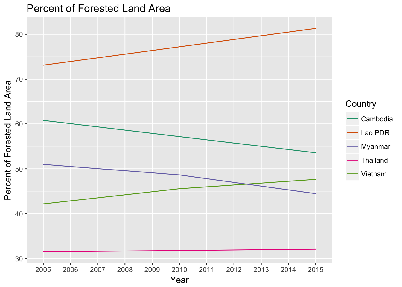

GDP_Plot<-ggplot(GDP_G,aes(x=Year,y=GDP,group=Country.Name))
  
GDP_Plot+
  geom_line(aes(color=factor(Country.Name)))+labs(title="GDP",y="GDP (US$)",color="Country")+
  scale_color_manual(values = plotcolors)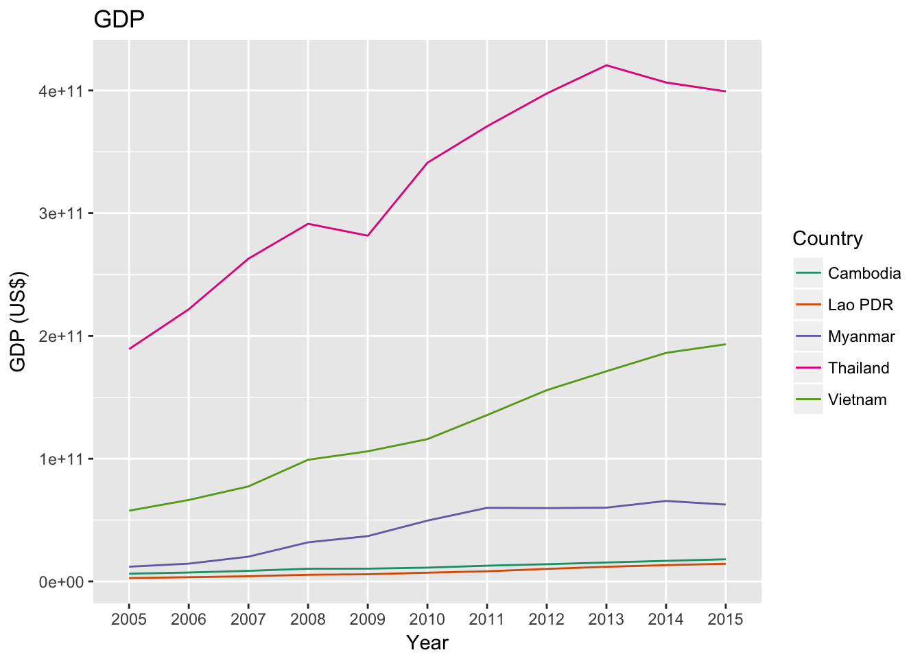

These plots display GDP and forested area trends through the ten year study period. They can be used as a reference to the more complicated plot below.

Forest Change and GDP

GDPF_colors=c("2005"="#a6cee3","2006"="#1f78b4","2007"="#b2df8a","2008"="#33a02c","2009"="#fb9a99","2010"="#e31a1c","2011"="#fdbf6f","2012"="#ff7f00","2013"="#cab2d6","2014"="#6a3d9a","2015"="#b15928")

GDPF_shape=c(15,16,17,18,7)

GDPF_plot+
  geom_point(aes(color=(as.character(Year)),shape=Country.Name,size=1))+
  labs(title="GDP and Forest Change (2005-2015)",shape="Country",color="Year",y="Percent of Forested Land Area")+
  scale_color_manual(values=GDPF_colors)+
  scale_shape_manual(values =GDPF_shape)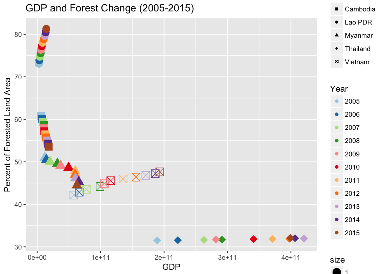

This plot displays Percent of Forested Area as a function of GDP. Countries are defined by shapes, and yearly values are defined by color. A discrete, qualitative color brewer was assigned to the values so distinctions in years by country can be deciphered. Light blue is assigned for 2005, and brown for 2015 to create highly contrasting colors to make trends more visible. As values move to the right it signifies a growth in GDP, as the values slump downwards it represents a loss in forested area.

Myanmar and Cambodia are experiencing a positive trend of GDP growth and an increase in forest loss. Thailand experiences a stagnating rate of deforestation but a staggering increase in GDP. Vietnam is increasing in both forested forested land and GDP. Laos experiences a small upward trend in GDP and a large gain in forested area.

World Map

The values of the global scale 10 year aggregate values are difficult to display due to such a wide range of values. Aggregate forest loss is displayed at 50% tree cover canopy density, the suggested global value according to the Global Forest Watch. As we can see below, indochina and Southeast Asia have relatively high percentage of ten year forest loss compared to the rest of the world. Note in both maps sustainable forestry and forest growth are not taken into consideration as it is impossible to calculate “net loss” or “net gain” with data provided (Hansen et.al.)

TCWebmap%>%
  addLegend(pal=pal,(values=~JN_join$tloss),title="Tree Cover Loss Percent (Ha)",position="bottomright")

Yearly Forested Land Area Loss (Ha)

WY_map%>%
  addLegend(pal=pal_05,(values=~join_06$Loss),title="Tree Cover Loss (Ha)",position="bottomleft")

Through time it is prevelant that each country in the region is experiencing an increase in total forest loss. Myanmar and Laos experience a consistent high level of forest loss year to year. Cambodia has negligible values of forest loss in 2005, but increases forest loss as time goes on. Thailand has a relatively consistent lower level of forest loss in the decadal interval.

References

Hansen, M. C., P. V. Potapov, R. Moore, M. Hancher, S. A. Turubanova, A. Tyukavina, D. Thau, S. V. Stehman, S. J. Goetz, T. R. Loveland, A. Kommareddy, A. Egorov, L. Chini, C. O. Justice, and J. R. G. Townshend. 2013. “High-Resolution Global Maps of 21st-Century Forest Cover Change.” Science 342 (15 November): 850–53. Data available on-line from: http://earthenginepartners.appspot.com/science-2013-global-forest.
World Bank, World Development Indicators (2016). GDP/Forest Area (% of land area)